Where to Put Level 1 and Level 2 Covariates in a Multilevel Model Stata

OS Programming algorithms

A Work on Scheduler schedules different processes to be assigned to the CPU supported uncommon scheduling algorithms. There are six popular treat scheduling algorithms which we are going to talk over in that chapter −

First-Come, First-Served (FCFS) Scheduling
Shortest-Job-Next (SJN) Scheduling
Priority Programming
Shortest Remaining Time
Round Robin(RR) Programming
Multiple-Rase Queues Scheduling

These algorithms are either non-preemptive or preemptive. Non-preemptive algorithms are designed so that once a process enters the running state, it cannot live preempted until it completes its allotted clip, whereas the preemptive scheduling is settled on antecedence where a scheduler may preempt a degraded priority gushing process anytime when a high precedence process enters into a ready state.

Freshman Come First Serve (FCFS)

Jobs are executed on first come, first serve basis.
It is a non-preemptive, pre-emptive scheduling algorithm.
Easy to empathise and put through.
Its implementation is supported FIFO queue.
Poor in performance as average wait time is high.

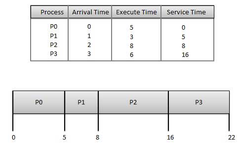
First Come First Serve Scheduling Algorithm

Wait meter of each process is as follows −

Process	Wait Time : Service Time - Arrival Time
P0	0 - 0 = 0
P1	5 - 1 = 4
P2	8 - 2 = 6
P3	16 - 3 = 13

Average Wait Time: (0+4+6+13) / 4 = 5.75

Shortest Job Next (SJN)

This is also called shortest job kickoff, Oregon SJF
This is a non-preemptive, pre-emptive scheduling algorithm.
Best approach to denigrate waiting time.
Easy to follow out in Batch systems where needed CPU time is known beforehand.
Impossible to follow out in synergistic systems where required CPU sentence is not known.
The processer should know in elevate how much time operation will take.

Given: Table of processes, and their Arrival time, Death penalty time

Process	Arrival Fourth dimension	Execution Time	Service Time
P0	0	5	0
P1	1	3	5
P2	2	8	14
P3	3	6	8

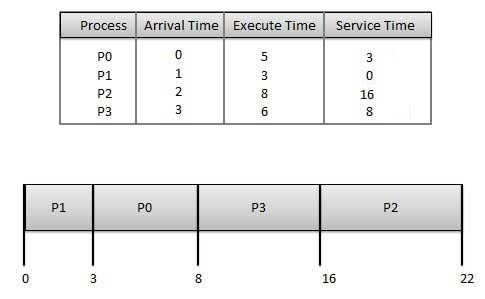
Shortest Job First Scheduling Algorithm

Wait time of to each one procedure is as follows −

Process	Waiting Time
P0	0 - 0 = 0
P1	5 - 1 = 4
P2	14 - 2 = 12
P3	8 - 3 = 5

Average Wait Time: (0 + 4 + 12 + 5)/4 = 21 / 4 = 5.25

Precedence Based Scheduling

Priority scheduling is a non-preemptive algorithmic rule and one of the most average scheduling algorithms in clutch systems.
Each process is allotted a priority. Process with highest anteriority is to live dead first and so on.
Processes with said priority are executed on inaugural come first served basis.
Priority can be decided supported memory requirements, time requirements or any other imagination requirement.

Disposed: Table of processes, and their Time of arrival, Execution time, and antecedence. Here we are considering 1 is the lowest priority.

Procedure	Arrival Time	Execution Time	Priority	Service Time
P0	0	5	1	0
P1	1	3	2	11
P2	2	8	1	14
P3	3	6	3	5

Priority Scheduling Algorithm

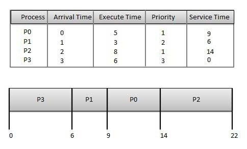
Wait time of each appendage is equally follows −

Process	Waiting Prison term
P0	0 - 0 = 0
P1	11 - 1 = 10
P2	14 - 2 = 12
P3	5 - 3 = 2

Average Wait Time: (0 + 10 + 12 + 2)/4 = 24 / 4 = 6

Shortest Remaining Clip

Shortest remaining time (SRT) is the preemptive version of the SJN algorithm.
The CPU is allocated to the job nearest to completion simply it can be preempted by a newer primed job with shorter prison term to completion.
Unbearable to implement in interactional systems where required Processor time is not noted.
IT is often used in batch environments where short jobs need to give penchant.

Round Robin Scheduling

Capitate Robin redbreast is the preemptive process scheduling algorithmic program.
Each process is provided a fix time to carry through, it is titled a quantum.
Once a process is dead for a given clock period, IT is preempted and other process executes for a given period of time.
Context switching is used to save states of preempted processes.

Round Robin Scheduling Algorithm

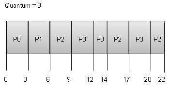
Wait clock time of each process is as follows −

Process	Waitress Time : Service Time - Arrival Time
P0	(0 - 0) + (12 - 3) = 9
P1	(3 - 1) = 2
P2	(6 - 2) + (14 - 9) + (20 - 17) = 12
P3	(9 - 3) + (17 - 12) = 11

Common Wait Time: (9+2+12+11) / 4 = 8.5

Multiple-Level Queues Programing

Multiple-flush queues are not an independent scheduling algorithm. They hold use of other existing algorithms to group and schedule jobs with common characteristics.

Multiple queues are maintained for processes with common characteristics.
Each queue up can have its own scheduling algorithms.
Priorities are assigned to each queue.

E.g., CPU-bound jobs can be regular in one queue and entirely I/O-in bonds jobs in some other queue. The Process Scheduler then alternately selects jobs from from each one queue and assigns them to the CPU based connected the algorithm assigned to the queue.